In this post I gonna write something to understand SVM. Thanks to Professor Francesco Orabona’s explain and most content of this post is learned from his course Convex Optimization.
What’s SVM
SVM, support vector machine, is a kind of machine learning model which can be used in classification and regression. In this blog, we will only illustrate how it works for binary classification.
First Step
Suppose we have a dataset \( {(x_i,y_i)} \), where \( x_i\in R^d \) and \( y_i \in {0,1} \). The classification problem is that we want to find a way to divide them perfectly. The easiest way is draw a hyperplane (which is a line when \( d=2 \) and a plane when \( d=3 \)). Now the problem is generally there is infinite ways to draw this plane. Which one is better?
Now let’s welcome SVM.
SVM argues that the best plane is the one which could create the largest margin.
Math
Now we will use math to make this problem more clear.
Hyperplane
A hyperplane can be defined as following:
\[W^Tx+b=0\]Notice that if we multiply a constant \(\lambda\) will not change the equation, which means the same hyperplane has infinite expressions. So here we restrict
\[\left\| W \right\| =1\]Distance
We will not use this equation directly. I put it here just because most blog about SVM will use this term.
The distance from a point \(x_0\) to a hyperplane \(W^Tx+b=0\) is
\[\frac{W^Tx_0+b0}{\left\| W \right\| }\]Margin
Margin is the smallest distance of all distances from data point to hyperplane. It’s illustrated by this example:
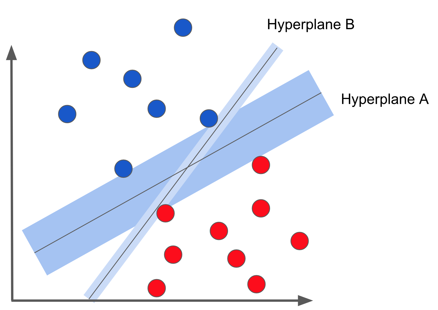
So in this example, there are two hyperplanes (in 2D they are two lines), the blue rectangles shows the margin. We can see that the margin corresponding to hyperplane A is bigger than that of hyperplane B.
SVM
Please be patient and in the end of this section, you will find the classic defination of SVM.
Remember we want to maximize the margin? In math, it’s simply
\[\text{max } M\]However, we need \(M\) to be the “margin”. So we add an restrict
\[y_iW^Tx_i \ge M\]Recall we already have a restrict:
\[\left\| W \right\| =1\]Now we can put every thing together like:
\[\begin{aligned} \text{max} \quad & M \\ s.t. \quad & y_iW^Tx_i \ge M, \forall i \\ & \left\| W \right\| =1 \end{aligned}\]Looks different from other blogs? Be patient, we will reach there.
Now let \(\tilde{W}=\frac{W}{M}\), we can get
\[\begin{aligned} \text{max} \quad & M \\ s.t. \quad & y_i \tilde{W}^Tx_i \ge 1, \forall i \\ & \left\| \tilde{W} \right\| =\frac{1}{M} \end{aligned}\]Now we get the margin “1” here, which is really where I don’t understand before. Let’s go further
Notice that \(\left| \tilde{W} \right| =\frac{1}{M}\), which tell us that \(M=\frac{1}{\left| \tilde{W} \right| }\). Let replace \(M\) with this equation and we will get
\[\begin{aligned} \text{max} \quad & \frac{1}{\left\| \tilde{W} \right\| } \\ s.t. \quad & y_i \tilde{W}^Tx_i \ge 1, \forall i \\ \end{aligned}\]See? One restrict is removed. Now the last step is replace max with min like:
\[\begin{aligned} \text{min} \quad & \left\| \tilde{W} \right\| \\ s.t. \quad & y_i \tilde{W}^Tx_i \ge 1, \forall i \\ \end{aligned}\]What else? Well, our purpose now is minimize \( \left| \tilde{W} \right| \), which is not quite differentiable on origin. So we can replace it with minimize \( \frac{1}{2}\left| \tilde{W} \right| ^2\). This will not change the optimal \( W^*\). The reason to add \(\frac{1}{2}\) is try to make the sequential step easier.
Now let’s list our question clearly here, which is one of the typical way to express the purpose of SVM
\[\begin{aligned} \text{min} \quad & \frac{1}{2}\left\| \tilde{W} \right\| ^2 \\ s.t. \quad & y_i \tilde{W}^Tx_i \ge 1, \forall i \\ \end{aligned}\]What’s next
- How to solve it: Lagrangian Dual and K.K.T. Conditions
- Kernel function: from linear to non-linear
- Tricks: multiple classification, regression, soft margin
- Python implement of SVM